数据去噪
DAS信号中的噪声主要有尖峰噪声、共模噪声、随机噪声和相干噪声。DASPy的数据去噪模块提供了 去尖峰噪声 、 去共模噪声 和 去随机噪声 三个功能,相干噪声可使用 波场分解 中提供的方法去除。
去尖峰噪声
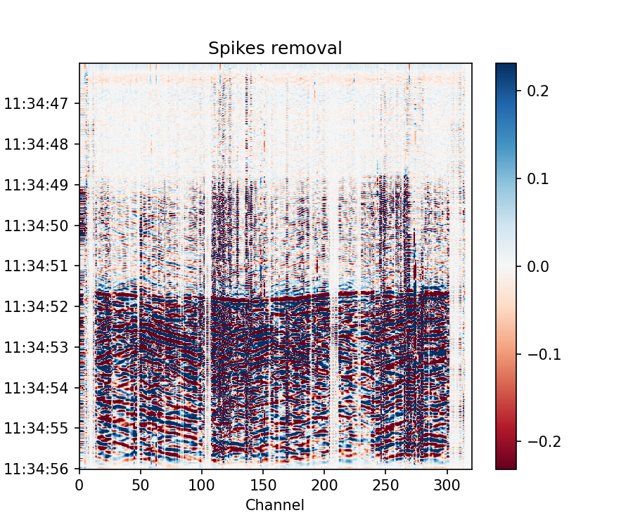
尖峰噪声表现为波形中异常大的振幅,通常是由激光频率漂移或激光噪声引起的。DASPy分别应用跨通道和跨时间中值滤波器,生成中值振幅谱图,并把振幅超过中值谱一定倍数的点识别为尖峰,然后用相邻通道的插值替换所有尖峰。
备注
示例数据为Stanford DAS-1记录的地震信号,可从 https://raw.githubusercontent.com/HMZ-03/DASPy-data/main/Stanford1_20180104_113058.566+0000.sgy 下载,并通过以下方式读取并预处理:
>>> from daspy import read, DASDateTime
>>> sec = read('Stanford1_20180104_113058.566+0000.sgy', ch2=320)
UserWarning: This data format segy doesn't include channel interval.
Please set Section.dx manually.
>>> sec.dx = 8
>>> sec.start_time = DASDateTime(2018, 1, 4, 11, 30, 58, 566000)
>>> origin_time = DASDateTime(2018, 1, 4, 11, 34, 44) # 发震时刻
>>> sec.bandpass(1, 20)
>>> sec.trimming(tmin=origin_time+2, tmax=origin_time+12)
>>> sec.plot(xmode='channel')
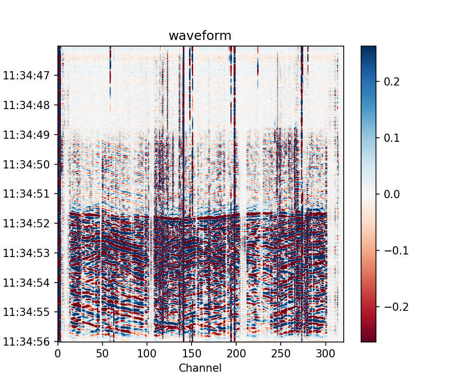
>>> sec.spike_removal()
>>> sec.plot(xmode='channel')
去共模噪声
共模噪声是由光电系统的振动产生的,并同时出现在所有信道上的同相噪声。DASPy采用波形的空间中值或平均值来获得共模噪声,计算信道记录和共模噪声的互相关系数,并从信道记录中去除共模噪声和互相关系数的乘积。
备注
示例数据为RAPID数据集的远海信道记录,可从 http://piweb.ooirsn.uw.edu/das/data/Optasense/NorthCable/TransmitFiber/North-C1-LR-P1kHz-GL50m-Sp2m-FS200Hz_2021-11-03T15_06_51-0700/North-C1-LR-P1kHz-GL50m-Sp2m-FS200Hz_2021-11-04T015902Z.h5 下载,并通过以下方式读取并预处理:
>>> import numpy as np
>>> from daspy import read
>>> sec = read('North-C1-LR-P1kHz-GL50m-Sp2m-FS200Hz_2021-11-04T015902Z.h5')
>>> sec.trimming(mode=0, xmin=18000, xmax=30000)
>>> sec.scale = 2 * np.pi / 2 ** 16 # 数据的缩放系数,见sec.headers['Acquisition']['Raw[0]']['attrs']['RawDataUnit']
>>> sec.phase2strain(1550.12 * 1e-9, 0.78, sec.headers['Acquisition']['Custom']['attrs']['Fibre Refractive Index']) # 将光相移转换为应变
>>> sec.bandpass(15, 27, detrend=True, taper=0.1)
>>> sec.trimming(tmin=sec.start_time+20, tmax=sec.start_time+30)
>>> sec.plot()
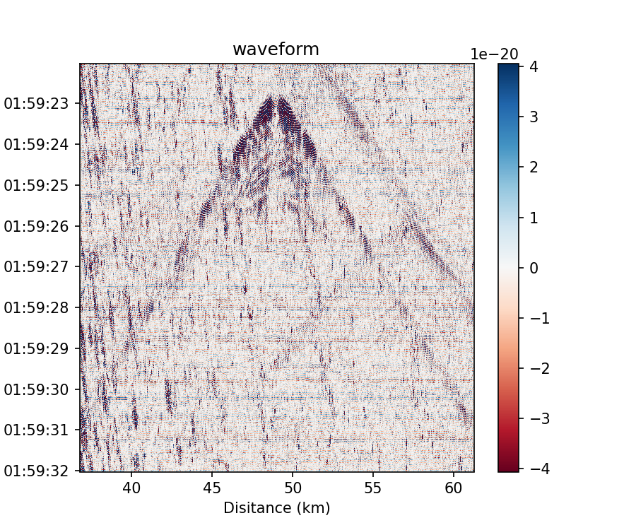
>>> sec.common_mode_noise_removal()
>>> sec.plot()

去随机噪声
DAS数据中的随机噪声主要是由采样误差和相位噪声等仪器缺陷引起的,DASPy使用曲线变换消除随机噪声:
备注
同 去尖峰噪声 使用的示例数据一致,此处使用去除尖峰噪声后的波形,并通过以下方式读取并预处理:
>>> from daspy import read, DASDateTime
>>> sec = read('Stanford1_20180104_113058.566+0000.sgy', ch2=320)
UserWarning: This data format segy doesn't include channel interval.
Please set Section.dx manually.
>>> sec.dx = 8
>>> sec.start_time = DASDateTime(2018, 1, 4, 11, 30, 58, 566000)
>>> sec.bandpass(1, 20)
>>> origin_time = DASDateTime(2018, 1, 4, 11, 34, 44) # 发震时刻
>>> sec.trimming(tmin=origin_time-10, tmax=origin_time+12)
>>> sec.spike_removal() # 数据中如有尖峰噪声,需要先去除
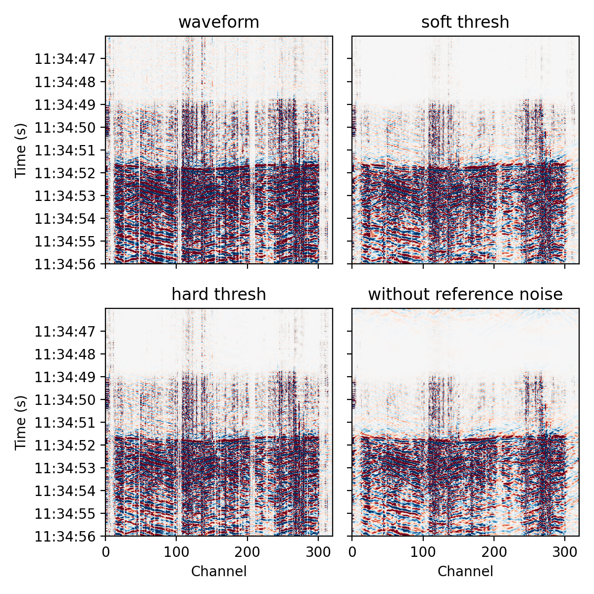
使用一段噪声记录作为噪声的基准,在曲波域以软阈值(默认)去除噪声:
>>> sec_eq = sec.copy().trimming(tmin=origin_time+2, tmax=origin_time+12) # 地震记录
>>> sec_ns = sec.copy().trimming(tmin=origin_time-10, tmax=origin_time) # 噪声记录
>>> sec_eq_soft = sec_eq.copy().curvelet_denoising(noise=sec_ns)
同样使用参考噪声记录,在曲波域以硬阈值去除噪声,可以使波形的绝对振幅不变小失真:
>>> sec_eq_hard = sec_eq.copy().curvelet_denoising(noise=sec_ns, soft_thresh=False)
没有可用的参考噪声记录时,函数会计算曲波系数的拐点以确定噪声的阈值,建议设置 pad=0 并调节 knee_fac 参数以减少人工伪影(不推荐此方法):
>>> sec_eq_knee = sec_eq.copy().curvelet_denoising(pad=0, knee_fac=0.1)
绘制原波形以及以上三种去噪的效果:
>>> import matplotlib.pyplot as plt
>>> fig, ax = plt.subplots(2, 2, figsize=(6,6), sharex=True, sharey=True, dpi=200)
>>> sec_eq.plot(ax=ax[0,0], xmode='channel', vmax=0.2, xlabel=False, colorbar=False)
>>> sec_eq_soft.plot(ax=ax[0,1], xmode='channel', vmax=0.2, xlabel=False, ylabel=False, colorbar=False, title='soft thresh')
>>> sec_eq_hard.plot(ax=ax[1,0], xmode='channel', vmax=0.2, colorbar=False, title='hard thresh')
>>> sec_eq_knee.plot(ax=ax[1,1], xmode='channel', vmax=0.2, ylabel=False, colorbar=False, title='without reference noise')
>>> plt.tight_layout()
>>> plt.show()